Examples of applications of explosion-proof electric motors
Installation of electric motors where flammable products are continuously used, processed or stored must comply with the highest safety standards to ensure the protection of life, machinery and the environment. Following the highest safety standards, WEG explosion-proof motors integrate high performance brakes. The perfect solution for equipment where quick safety stops are required, as well as precise positioning with safety in hazardous areas such as zone 1 and zone 2. WEG Exd motors with brakes are available in versions: standard efficiency (EFF2), efficiency Superior (EFF1) and Superior Efficiency (more than EFF1) and certified for performance with frequency inverters.

Standard features of explosion-proof electric motor
-
- Three-phase, multi-voltage, IP55, TEFC
- Output power: 0.37 to 330 kW
- Frame: 90S to 355M/L
- Voltage: 220-240/380-415V (up to 100L) / 380-415/660V (from 112M and up))
- Class “F” insulation (T=80K)
- Continuous duty: S1
Explosion-proof electric motor design
- Ambient temperature: 40 degrees Celsius, in 1000 square meters
- Squirrel cage rotor/aluminum diecast
- Lip seals on both end shields
- AISI 316 stainless steel plate
- Dimensions according to IEC 60072
- Performance characteristics in accordance with IEC 60034-30
- Nipple from frame 225S/M and above
- Metric threaded cable entries on terminal box
- Thermistor (1 per phase) for all frames
- Suitable for inverter applications*
- Color: RAL 5010
* For more details about inverter performance, please contact our technical support.
Optional options of explosion-proof electric motor
- Degree of protection: IP56, IP65 or IP66 (W)
- Bearing seal:
- Oil seal
- Labyrinth and W3seal taconite seals for 90S and higher frames
- Thermal protection:
- Thermistor: Frame 132M and below
- Thermostats
- RTD-PT 100
- Space heaters
- Design H
- Class “H” insulation.
- Roller bearing for frame 160M and above
More options are available upon request
Classification of explosion-proof electric motor
IEC standard of explosion-proof electric motor
Region 1; Group IIB
CENELEC standard for explosion-proof electric motor
- Group IIB; Category 2
- Classification in zone 1 means that the motor is also suitable for a load in zone 2
- Region 1 shows a worse operating condition than Region 2.
- The same applies to groups and categories: Ex d and Ex de motors are also suitable for operation in group IIA and category 3.
Certificates of explosion-proof electric motors
In Europe, WEG explosion-proof motors according to the ATEX directive 94/9/EC with PTB certificate and CESI-certified product – Centro Elettrotecnico Spimentale Italiano SPA CESI certificates for explosion-proof in the “d” and “de” flameproof enclosure according to / EN50018 as follows:
Ex d – explosion-proof motors (temperature class T4)
Ex de – explosion-proof motors with increased safety terminal box (temperature class T4)
Explosion-proof electric motor frame certificate number
- 90-100 CESI 01 ATEX 096
- 112-132 CESI 01 ATEX 097
- 160-200 CESI 01 ATEX 098
- 225-250 CESI 01 ATEX 099
- 280-315 CESI 01 ATEX 100
Explosion-proof electric motor standard
In Europe, WEG explosion-proof motors according to the ATEX directive 94/9/EC with PTB certificate and CESI-certified product – Centro Elettrotecnico Spimentale Italiano SPA CESI certificates for explosion-proof in the “d” and “de” flameproof enclosure according to / EN50018 as follows:
Ex d – explosion-proof motors (temperature class T4)
Ex de
Electric motor – electrical energy mechanics. Energy conversion machine
It has DC and AC types.
For direct current, which can adjust the rotation frequency effectively and uniformly. K advantage is considered.
alternating current. Synchronous electric motor (electric motor whose rotation frequency depends on current frequency), asynchronous electric motor (electric motor whose rotation frequency decreases with increasing load) and collector electric motor. K. Belongs to. In practice, asynchronous E. K. widespread. Making such an engine is simple and reliable.
Asynchronous E. The main disadvantage of k: it uses a lot of reactive power. If it is necessary to change the rotation frequency to uniform,
direct current. K. Sometimes the collector AC E. K. is used E. The k power ranges from a tenth of a watt to tens of megawatts.
K. In industry, in transportation, in life, etc. It is widely used in industries.
Electric motor
An electric motor is a machine that converts electrical energy into mechanical energy that can be used to move tools. Electric motors are divided into two categories: direct current and alternating current. In addition to conventional motors that provide rotary motion, there are also linear motors.
History and development of electric motor
original

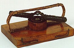
The conversion of electrical energy into mechanical energy through electromagnetism was first performed by the British scientist Michael in 1821. Faraday showed. At the moment when a current flows through the conductor, the conductor makes a rotational movement around the magnet.
This electric motor is the simplest version of the homopolar motor. The improved shape of this wheel is Barlow. Due to their original construction, these electric motors could only be used for demonstration purposes. They are unsuitable for any practical use.
In 1827, Hungarian Anius Yedlik began experimenting with electromagnetic rotating devices, which he called the magnetic lightning rotor. He was using this device for educational purposes in college. In 1828, he demonstrated the first device that includes the three main components of a DC motor: stator, rotor, and commutator. His electric motor also had no practical use and after that his knowledge was forgotten.
The first electric motors
The first displacement DC motor capable of moving tools was invented in 1832 by the British scientist William Sturgeon. American built following the work of Sturgeon, a DC motor improved by Thomas Davenport to use it for practical purposes. His electric motor, which was patented in 1837, rotated at a speed of 600 revolutions per minute and powered light machine tools and printing presses.
Due to the high cost of the zinc electrodes used in the batteries, his engine was not a commercial success and Davenport went bankrupt. Many inventors followed Sturgeon and Davenport in developing the electric motor, but all faced the same problem: the high energy cost of batteries.
The modern DC motor was accidentally discovered in 1873 by Hippolyte Fontaine and Zénobe Gramme. They were connected in parallel, when two dynamo’s were heated, one of the dynamo’s acted as a motor, driven electrically by the other. In this way, the hot car became the first successful industrial electric motor.
In 1888, Nikola Tesla invented the first practical induction motor powered by a two-phase AC power supply. Tesla continued his work with the AC motor in the following years at Westinghouse. Independent of Tesla’s research, Mikhail Doliwo-Dobrowolski developed the squirrel armature three-phase asynchronous motor at the same time (1888).
Electric motor operation
The operation of an electric motor is based on electromagnetism. The motor consists of a stator and a rotor that can rotate in the stator. At least one of these two is designed as an electromagnet. Depending on the type of motor, the other can be made as a permanent magnet, electromagnet, or just magnetic material. The rotor starts rotating due to the force of the magnetic poles on each other or due to induction.
Every electric motor also works as a dynamo, the rotating motor produces electricity. This flow is opposite to the supply flow.
The high resistance of an electric motor does not have to be high and so current will flow when it is turned on. The engine now runs and acts as an alternator. The generated current flows in the opposite direction and the net current becomes less. Ideally, the motor would run at full speed, the generated current would be equal (but opposite) to the supply current, and no current would flow at all. In practice, especially when the motor is under load, the motor rotates a little slower, so that the generated current is slightly less than the supplied current.
If the motor is held so that it cannot rotate, the supply current may cause the motor to smoke.
Therefore, a higher current flows through the motor during starting than during operation (starting current). Therefore, a heavy motor is sometimes started at a lower voltage, often with a star-delta connection, and connected to a slow-blow fuse.

Electric motor template
DC motor with brush
A brushed DC motor requires the rotor poles to be reversed every half turn (or more often, the collectors if the rotor and stator consist of more than two parts) to allow the motor to rotate. This polarity change is caused by the commutator and carbon brushes. If the direction of the current passing through it is reversed, the motor will continue to rotate.
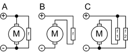
B: Series
C: Compound
The motor can be designed as a series or shunt motor, where the field and rotor windings are connected in series and parallel, respectively. A combination of both is also possible, the so-called hybrid engine.
Brushless electric motor
There are also electric motors where the commutation is electronically controlled. These brushless electric motors do not have carbon brushes that prevent sparks and wear (the problem of brush motors). Such a motor is also called an ECM motor (Electronically Commutated Motor).

Thermal development of electric motor
The most common cause of electric motor failure is excessive heat generation. The motor overheats, which can cause the bearings to fail, the windings to short out, or the magnets to permanently demagnetize and lose power. [2]
AC electric motor
A three-phase AC motor can be very simple in construction because the commutator/carbon brush structure can be dispensed with. This is about the squirrel cage engine. But carbon brushes (rotor) are used in sliding ring armature motor. The speed of the squirrel cage motor can be easily controlled by a frequency controller.
Applications
An electric motor is present in many devices, and it has become so obvious that people no longer realize that it contains an electric motor, or that the word electric motor is not even fully present in the description of a device. Examples:
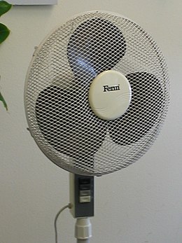
- Household appliances: washing machine, dryer, refrigerator, vacuum cleaner, sewing machine, shaver, electric toothbrush, hair dryer, fan, some watches
- Kitchen appliances: food processor, juicer, hand mixer, blender, hand blender, coffee grinder, hood, microwave, ice maker
- DIY tools: drill, planer, sander, jigsaw
- Gardening tools: leaf blower, chainsaw, hedge trimmer, scarifier, lawn mower, rotary mower
- Electronics: computer, hard disk, printers (inkjet printer, laser printer), flatbed scanner, copier, fax machine, electric typewriter
- Toys: electric model train, airplane model, helicopter model, robot, drone
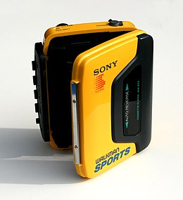
- Audio and visual equipment: gramophone (player), jukebox, CD player, VCR, cassette recorder, camera, video camera, walkman
- Automatic in public buildings (shops, offices, hospitals, libraries): sliding doors, revolving doors, elevators, escalators, floor polishers
- Houses: mechanical ventilation, stair lifts, garage doors, awnings, shutters, fences and gates.
Different professions have their own equipment: baker (bread slicer, kneading machine), butcher (meat slicer, meat grinder), dentist (dental drill), scissors sharpener (electric grinder). In the medical department, ventilators, heart and lung devices, peristaltic pumps, insulin pumps, and centrifuges are used.
In addition, many means of transportation are powered by electric motors, for example trains, trams, electric cars, electric scooters and motorcycles, electric scooters and wheelchairs, electric bicycles, Segways, hoverboards, and ships such as the Whisper Boat. , submarine, electric speed. The boat [3] works, there are also experimental cars, buses and airplanes with electric motors powered by fuel cells. The starter motor of a car with a combustion engine (gasoline/diesel) is also an electric motor and is used to start the combustion engine. This modern luxury car is equipped with about 15 electric motors: starter motor, to open and close four windows, adjust and fold in/out two exterior mirrors, 2 or 3 wipers, windshield washer pump, power steering, Air. Air conditioning and CD player. player
is used Also, in the 3-phase motor industry, it is mainly used to drive pumps, compressors, conveyor belts, cranes and other lifting devices, agitators in tanks, air conditioning installations, combustion air and flue gas transmission, etc. The motor specifically produces electricity when it is turned on. It will be a big startup stream. This is very stressful for the power grid. Sometimes this even causes an instant softening of the electric light of the environment. In order to prevent or smooth these “peaks”, such an engine is started with a starting device.
Magnetic field
| Articles about |
| Electromagnetism |
|---|
 |
|
|
Electrostatic
|
|
Static magnetism
|
|
Electrodynamics
|
|
electricity network
|
|
Covariance formula
|
|
Scientists
|
|
A magnetic field is a vector field that describes the magnetic effect on moving electric charges, electric currents. [1] : ch1 [2] and magnetic material, the moving charge in the magnetic field experiences a force perpendicular to its speed and the magnetic field. [1] : ch13 [3] : 278The magnetic field of a permanent magnet attracts or repels ferromagnetic materials such as iron and other magnets. Additionally, a non-uniform magnetic field exerts small forces on “non-magnetic” materials through three other magnetic effects: paramagnetism, diamagnetism, and antiferromagnetism, although these forces are usually so small that they can only be detected with laboratory equipment. Magnetic fields surround magnetic materials and are created by electric currents such as those used in electromagnets and time-varying electric fields. Since both the strength and direction of a magnetic field may vary with location, it is mathematically described by a function that assigns a vector to any point in space. vector field
In electromagnetics, the term “magnetic field” is used for two separate but closely related vector fields denoted by the symbols B and H. In the International System of Units, the unit is H, the strength of the magnetic field, ampere per meter (A/m). [4] : 22 units of B is the magnetic flux density, tesla (in SI base units: kg/s 2/ampere), [4] : 21 which is equivalent to Newton/meter/ampere. H and B differ in the way magnetic is calculated. In a vacuum, these two fields are connected through the permeability of the vacuum. B / m 0 = H ; But in a magnetic material, the values on each side of this equation are different from the magnetic field of the material.
 ; But in a magnetic material, the values on each side of this equation are different from the magnetic field of the material.
Magnetic fields are produced by the movement of electric charges and inherent magnetic moments of fundamental particles related to their fundamental quantum property, i.e. their spin. [5] [1] : ch1 Magnetic fields and electric fields are related and both components of the electromagnetic force are one of the four fundamental forces of nature.
Magnetic fields are used throughout modern technology, especially in electrical and electromechanical engineering. Rotating magnetic fields are used in both electric motors and generators. The interaction of magnetic fields in electrical devices such as transformers is conceptualized and investigated as magnetic circuits. Magnetic forces provide information about charge carriers in a material through the Hall effect. The Earth produces its own magnetic field that protects the Earth’s ozone layer from the solar wind and is important in navigation using a compass.
Description
The force on an electric charge depends on its location, speed and direction. Two vector fields are used to describe this force. [1] : ch1 is the first electric field that describes the force acting on a fixed charge and shows a component of force independent of motion. In contrast, the magnetic field describes a component of force that is proportional to the speed and direction of the charged particles. [1] : ch13 The field is defined by the Lorentz force law and is perpendicular to both the motion of the charge and the force it experiences at any instant.
Different, but closely related, exist two vector fields, both sometimes called “magnetic fields”, written B and H. [Note 1] While the best names for these fields and the precise interpretation of what these fields represent have been the subject of long-standing debate, there is broad agreement about how fundamental physics works. [6] Historically, the term “magnetic field” was reserved for H while other terms were used for B, but many recent textbooks use the term “magnetic field” to describe B or They use H instead. [note 2] There are many alternative names for both (see sidebar).
Square B

| Alternative names for B [7] |
|---|
|
The magnetic field vector B at any point can be defined as the vector that, when used in the Lorentz force law, correctly predicts the force on the charged particle at that point: [9] [10] : 204
Law of Lorentz force (vector, SI units) F = q E + q (v × b)

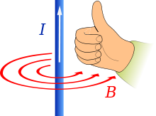
Here, F is the force on the particle, q is the particle’s electric charge, v is the particle’s velocity, and x represents the cross product. The direction of the force acting on the load can be determined by a notation called the right-hand rule (see figure). [Note 3] Using the right hand, place the thumb in the direction of the current, and the fingers in the direction of the magnetic field, the force resulting from the applied charge is outward from the palm. The force acting on a negatively charged particle is in the opposite direction. If both the velocity and the load are reversed, the direction of the force remains the same. Because of this, measuring the magnetic field (by itself) cannot tell whether a positive charge is moving to the right or a negative charge is moving to the left. (Both of these produce the same current.) Alternatively, a magnetic field combined with an electric field can distinguish between the two, see the Hall effect below.
The first term in the Lorentz equation is from electrostatic theory and says that a particle of charge q experiences an electric force in an electric field E:

The second term is the magnetic force: [10]

Using the cross definition, the magnetic force can also be written as a scalar equation: [9] : 357

where F is magnetic, v and B are the scalar magnitudes of their respective vectors and θ is the angle between the particle velocity and the magnetic field. Vector B is defined as the vector field necessary to correctly describe the motion of a charged particle by the law of Lorentz force. In other words, [9 :173-4]
[T] The command “Measure the direction and magnitude of the vector B at such a location” calls the following operation: Take a particle with a known charge q. Measure the force on q at rest to determine E. Then measure the force on the particle when its speed is v. Repeat with v in the other direction. Now find a B that satisfies the Lorentz force law with all these results – that is, the magnetic field at the desired location.
The field B can also be defined by the moment on a magnetic dipole, m. [11] : 174
Magnetic moment (vector, SI units) t = m × b

SI unit B (symbol: Tesla T). [Note 4] Gaussian unit-cgs B (symbol: is Gauss G). (The conversion of 1 T ≘ 10000 G. [12] [13] ) One nanotesla corresponds to 1 gamma (symbol: γ). [13]
Square H
| Alternative names for H [7] |
|---|
|
The magnetic field H is defined as: [10] : 269 [11] : 192 [1] : ch36
Definition of H field (vector form, SI units) H ≡ 1 m 0 b-m

where m is 0 vacuum permeability and M is magnetic vector. In vacuum, B and H are proportional to each other. Inside a material they are different (see H and B inside and outside magnetic materials). The SI unit of field H is ampere per meter (A/m), [14] and the CGS unit is Orsted (Oe). [12] [9]: 286
 is 0 vacuum permeability and M is magnetic vector. In vacuum, B and H are proportional to each other. Inside a material they are different (see H and B inside and outside magnetic materials). The SI unit of field H is ampere per meter (A/m), [14] and the CGS unit is Orsted (Oe). [12] [9]:
 measurement
The instrument used to measure the local magnetic field is known as a magnetometer. Important categories of magnetometers include induction magnetometers (or search coil magnetometers) that measure only changing magnetic fields, rotating coil magnetometers, Hall effect magnetometers, NMR magnetometers, SQUID magnetometers, and flux magnetometers. The magnetic fields of distant astronomical objects are measured through their effect on local charged particles. For example, electrons spiraling around a field line produce synchrotron radiation, which is detectable in radio waves. The best accuracy for measuring the magnetic field by gravity B was obtained at 5 aT (5 x 10-18 probe T). [15]
Visualization

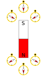
Right: Compass needles point in the direction of the local magnetic field, toward the magnet’s south pole and away from its north pole.
The field can be visualized by a set of magnetic field lines, which follow the direction of the field at any point. Lines can be constructed by measuring the strength and direction of the magnetic field at a large number of points (or anywhere in space). Then, mark each location with an arrow (called a vector) pointing in the direction of the local magnetic field with a magnitude proportional to the magnetic field strength. Then the connection of these arrows forms a set of magnetic field lines. The direction of the magnetic field at any point is parallel to the direction of the adjacent field lines, and the local density of the field lines can be considered proportional to its strength. Magnetic field lines are like streamlines in a fluid flow, in that they represent a continuous distribution, and the varying resolution of the lines indicates more or less.
The advantage of using magnetic field lines as a representation is that many of the laws of magnetism (and electromagnetism) can be fully and concisely expressed using simple concepts such as the “number” of field lines in a plane. These concepts can be quickly “translated” into their mathematical form. For example, the number of field lines crossing a given surface is the surface integral of the magnetic field. [9] : 237
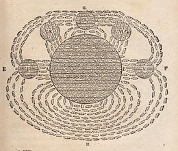
Various phenomena display magnetic field lines as if the field lines were physical phenomena. For example, iron filings placed in a magnetic field form lines that correspond to “field lines”. [note 5] Magnetic field “lines” are also visually displayed in auroras, where dipolar interactions of plasma particles create visible streaks of light that align with the local direction of the Earth’s magnetic field. be.
Field lines can be used as a qualitative tool to visualize magnetic forces. In the ferromagnetism of materials such as iron and plasma, magnetic forces can be understood by imagining that field lines exert a tension (like a rubber band) along their length and a compression perpendicular to their length on adjacent field lines. The “opposite” poles of a magnet attract because they are connected by many field lines. “Like” poles are repelled because their field lines do not meet, but are parallel and push against each other.
Magnetic field of permanent magnets
Permanent magnets are objects that generate their own permanent magnetic fields. They are made of ferromagnetic materials such as iron and nickel that are magnetized and have north and south poles.
The magnetic field of permanent magnets can be very complex, especially near the magnet. The magnetic field of a small direct magnet [Note 6] is proportional to the magnet’s strength (called the magnetic dipole moment m ). The equations are non-trivial and also depend on the distance from the magnet and the direction of the magnet. For simple magnets, m is in the direction of a line drawn from the south to the north pole of the magnet. Rotating a bar magnet is equivalent to rotating it 180 degrees.
By modeling them as a collection of many small magnets called dipoles, the magnetic field of larger magnets can be obtained. The magnetic field produced by the magnet is the net magnetic field of this dipole. Any net force on the magnet is the sum of the forces on the individual poles.
There were two simplified models for the nature of these dipoles. These two models produce two different magnetic fields H and B. However, outside of a substance, the two are the same (up to a multiplicative constant) so that in many cases the distinction can be ignored. This is especially true of magnetic fields, such as those caused by electric currents that are not produced by magnetic materials.
A true model of magnetism is more complex than either of these models. Neither model fully explains why materials are magnetic. The unipolar model has no experimental support. Ampere’s model explains some, but not all, of a material’s magnetic moment. As Ampère’s model predicts, the motion of electrons in an atom is connected to the orbital magnetic dipole moments of those electrons, and these orbital moments contribute to the magnetism observed at the macroscopic level. However, the motion of the electrons is not classical, and the spin magnetic moment of the electrons (which is not accounted for by either model) also makes a significant contribution to the total moment of the magnets.
Magnetic pole model

Historically, early physics textbooks modeled the forces and torques between two magnets due to the magnetic poles repelling or attracting each other in the same way as the Coulomb force between electric charges. At the microscopic level, this model conflicts with experimental evidence, and the polar model of magnetism is no longer the usual way to introduce this concept. [10] : 204 However, due to its mathematical simplicity, it is still sometimes used as a macroscopic model for ferromagnetism. [16]
In this model, a magnetic field H is generated by fictitious magnetic charges spread over the surface of each pole. These magnetic charges are actually related to the magnetic field M. Therefore, the field H is similar to the electric field E, which starts with a positive electric charge and ends with a negative electric charge. Therefore, near the North Pole, all H field lines point toward the North Pole (either inside or outside the magnet), while near the South Pole, all H field lines point toward the South Pole (either inside or outside the magnet). are located Also, a north pole feels a force in the direction of the H field, while the force on a south pole is opposite to the H field.
In the magnetic pole model, the initial magnetic dipole m is formed by two opposite magnetic poles with the pole strength qm, which are separated by a small distance vector d, so that m = qm d. The magnetic pole model correctly predicts the field H inside and outside the magnetic material, especially the fact that H is opposite to the magnetic field M inside a permanent magnet.
Since this model is based on the fictitious idea of magnetic charge density, the pole model has some limitations. Magnetic poles cannot exist apart from each other like electric charges, but are always in north-south pairs. If a magnetic object is split in half, a new pole appears on the surface of each piece, so each has a pair of complementary poles. The magnetic pole model does not take into account the magnetization produced by electric currents as well as the intrinsic connection between angular momentum and magnetization.
The polar model usually treats magnetic charge as a mathematical abstraction rather than a physical property of particles. However, a magnetic monopole is a hypothetical particle (or class of particles) that physically has only one magnetic pole (either a north pole or a south pole). In other words, it has a “magnetic charge” similar to an electric charge. Magnetic field lines begin or end on magnetic monopoles, so if they exist, they are exceptions to the rule that magnetic field lines neither begin nor end. Some theories (such as grand unified theories) have predicted the existence of magnetic monopoles, but none have been observed so far.
Amprin ring model


In the model developed by Ampere, the basic magnetic dipole that makes up all magnets is a sufficiently small Ampere loop with current I and loop area A. The dipole moment of this ring is m = IA.
These magnetic dipoles produce a magnetic B field.
The magnetic field of a magnetic dipole is shown in Fig. Externally, an ideal magnetic dipole is identical to an ideal electric dipole of the same strength. Unlike an electric dipole, a magnetic dipole is correctly modeled as a current loop with current I and area a. Such a current loop has a magnetic moment

where the direction m is perpendicular to the area of the ring and depends on the flow direction using the right-hand rule. An ideal magnetic dipole is modeled as a real magnetic dipole with its area a reduced to zero and its current I increased to infinity, so that the product m = Ia is bounded. This model clarifies the relationship between angular momentum and magnetic moment, which is the basis of the Einstein-Dahas effect of rotation by magnetization and its inverse, the Barnett effect or magnetization with rotation. [17] Faster rotation of the loop (in the same direction) for example, increases the current and thus the magnetic moment.
Interaction with magnets
force between magnets
Determining the force between two small magnets is very complicated because it depends on the strength and direction of both magnets and their distance and direction relative to each other. This force is especially sensitive to the rotation of the magnets due to the magnetic moment. The force on each magnet depends on its magnetic moment and the magnetic field [note 7] of the other.
To understand the force between magnets, it is helpful to examine the magnetic pole model presented above. In this model, the H field of one magnet pushes and pulls both poles of the second magnet. If this field H is the same at both poles of the second magnet, there is no net force on that magnet because the force is opposite for opposite poles. However, if the magnetic field of the first magnet is non-uniform (such as H near one of its poles), each pole of the second magnet sees a different field and is subjected to a different force. This difference in the two forces moves the magnet in the direction of increasing the magnetic field and may also cause a net torque.
This is a specific example of a general rule that magnets are attracted to areas of higher magnetic field (or repelled depending on the orientation of the magnet). Any non-uniform magnetic field, whether caused by permanent magnets or electric currents, thus exerts a force on a small magnet.
The details of Amprin’s loop model are different and more complicated, but the result is the same: that magnetic dipoles are attracted/repelled to regions of higher magnetic field. Mathematically, the force acting on a small magnet that has a magnetic moment m due to the magnetic field B is: [18] : Eq. 11.42

where the gradient ∇ is the change in the quantity of m · B per unit distance and the direction of the maximum increase of m · B. The dot product m · B = mB cos( θ ), where m and B represent the magnitude of vectors m and B, and θ is the angle between them. If m is in the same direction as B, the dot product is positive and the dot gradient is “uphill” pulling the magnet higher up into regions of larger B field (more precisely m · B ). This equation is only valid for magnets of size zero, but is often a good approximation for not very large magnets. The magnetic force on larger magnets is determined by dividing them into smaller areas, each of which has m, and then the forces acting on each of these very small areas are collected.
Magnetic moment on permanent magnets
If two similar poles of two separate magnets are brought close to each other and one of the magnets is allowed to rotate, it immediately rotates to align itself with the first magnet. In this example, the magnetic field of the permanent magnet creates a magnetic moment on the magnet, which is free to rotate. This magnetic moment τ tends to align the magnet poles with the magnetic field lines. Therefore, the compass rotates to align itself with the Earth’s magnetic field.


According to the polar model, two equal and opposite magnetic charges that experience the same H also experience equal and opposite forces. Since these equal and opposite forces are located in different places, a torque proportional to the distance (perpendicular to the force) is created between them. Defining m as the pole strength times the distance between the poles, this leads to τ = μ 0 m H sin θ , where μ 0 is a constant called the vacuum, measuring 4π × 10–7 permeability V · s / (A · m) and θ is the angle between H and m.
Mathematically, the torque τ on a small magnet is proportional to both the applied magnetic field and the magnetic moment m of the magnet:

where x represents the vector cross product. This equation contains all the qualitative information above. There is no torque on the magnet if m is the direction of the magnetic field, because the cross product is zero for two vectors that are in the same direction. In addition, all other directions feel a torque that twists them towards the direction of the magnetic field.
Interaction with electric currents
The flow of electric charges both creates a magnetic field and feels a force due to magnetic B fields.
Magnetic field caused by moving charges and electric currents
All moving charged particles produce a magnetic field. Moving point charges, such as electrons, produce complex but well-known magnetic fields that depend on the charge, velocity, and acceleration of the particles. [19]
Magnetic field lines form concentric circles around a current-carrying cylindrical conductor, such as a length of wire. The direction of such a magnetic field can be determined using the “right-hand rule” (see figure on the right). The strength of the magnetic field decreases with distance from the wire. (For a wire with infinite length, the strength is inversely proportional to the distance.)

Bending a current-carrying wire in a loop concentrates the magnetic field inside the loop while weakening it outside. Bending a wire in several closely spaced loops to form a coil or “solenoid” enhances this effect. A device formed around a functioning iron core may act as an electromagnet and generate a strong and well-controlled magnetic field. An infinite cylindrical electromagnet has a uniform magnetic field inside and no magnetic field outside. An electromagnet of finite length produces a magnetic field that is similar to the magnetic field produced by a uniform permanent magnet whose strength and polarity are determined by the current flowing through the coil.
The magnetic field produced by a constant current I (a constant flow of electric charges, in which the charge is not accumulated or discharged at any point) [Note 8] is described by the Biot-Savart law: [20]: 224
 w i r e d ℓ × r ^ r 2,

where the integral sum over the length of the wire where the vector d ℓ is the line vector element with the same direction as the current I, μ 0 is the magnetic constant, r is the distance between the location d ℓ and the location where the magnetic field is calculated, and r is a The unit vector is in the r direction. For example, for a sufficiently long and straight wire, this becomes:

where r = | | . The tangent direction to a circle is perpendicular to the wire according to the right-hand rule. [20] : 225
A slightly more general way [21] [note 9] to relate the current I to the field B is through Ampere’s law:
 to the field B is through Ampere’s law:

where is the line integral over any arbitrary loop and i enc is the current enclosed by that loop. Ampere’s law is always valid for steady currents and can be used to calculate the B-field for certain highly symmetrical situations such as an infinite wire or an infinite solenoid.
 is the current enclosed by that loop. Ampere’s law is always valid for steady currents and can be used to calculate the B-field for certain highly symmetrical situations such as an infinite wire or an infinite solenoid.
Ampere’s law, in a modified form that accounts for time-varying electric fields, is one of Maxwell’s four equations that describe electricity and magnetism.
Force on moving loads and current
The force on the charged particle of the electric motor
A charged particle moving in a field B experiences a lateral force that is proportional to the strength of the magnetic field, the component of the velocity perpendicular to the magnetic field, and the charge of the particle. This force is known as the Lorentz force and is given by

where F is the velocity force, q is the electric charge of the particle, v is the moment of the particle, and B is the magnetic field (in tesla).
The Lorentz force is always perpendicular to both the velocity of the particle and the magnetic field that creates it. When a charged particle moves in a static magnetic field, it follows a helical path where the axis of the helix is parallel to the magnetic field and where the velocity of the particle remains constant. Since the magnetic force is always perpendicular to the motion, the magnetic field cannot do anything on an individual charge. [22] [23] It can only work indirectly, through an electric field created by a changing magnetic field. Non-primitive It is often claimed that the magnetic force can do work on a magnetic dipole or charged particles whose motion is constrained by other forces, but this is false [24] because the work in these cases is done by electric forces. Charges deflected by a magnetic field.
The force on the current carrying wire
The force on the current-carrying wire is as expected similar to the force on the moving charge because the current-carrying wire is a collection of moving charges. A current-carrying wire feels a force in the presence of a magnetic field. Lorentz force in macroscopic flow is often known as Laplace force. Consider a conductor of length ℓ, cross-section A and charge q due to electric current i. If this conductor is placed in a magnetic field with a magnitude B of an angle θ that creates charges in the conductor at a speed, the force exerted on a single charge q is equal to

Therefore, for N charges where

is the force applied to the conductor

where i = nqvA .
The relationship between H and B
The formulas obtained for high magnetic field are correct when dealing with total current. A magnetic material placed inside a magnetic field produces itself, a finite current that can be challenging to calculate. (This limited current is due to the sum of the atomic-sized current loops and the spin of subatomic particles such as electrons that make up matter.) The H field, as defined above, helps determine this limited current. It helps to introduce the concept of magnetism, but to see how, first.
Magnetization
The vector magnetic field M indicates the intensity of magnetization of a region of the material. It is defined as the net magnetic dipole moment per unit volume of that area. Therefore, the magnetization of a uniform magnet is a material constant that is equal to the magnetic moment m of the magnet divided by its volume. Since the SI unit of magnetic moment is A⋅m 2 , the SI unit of magnetic M is ampere-meter, which is the same as field H.
The magnetic field M of a region is in the direction of the average magnetic dipole moment in that region. Therefore, the magnetic field lines start near the magnetic south pole and end near the magnetic north pole. (There is no magnetism outside the magnet.)
In the amperine ring model, the magnetization is due to the combination of many small amperine rings to form a current called a finite current. Therefore, this limited current is the source of the magnetic field B caused by the magnet. According to the definition of magnetic dipole, the magnetic field follows a law similar to Ampere’s law: [25]

where the integral is a line integral over each closed loop and I b is the finite current enclosed by that closed loop.
In the magnetic pole model, magnetization starts from the magnetic poles and ends at them. Therefore, if a given region has a net positive “magnetic pole strength” (relative to the north pole), it has more magnetic field lines entering it than leaving it. Mathematically, this is equivalent to:

where the integral is a closed surface integral over the closed surface S and q M is the “magnetic charge” (in units of magnetic flux) enclosed by S. (A closed surface completely surrounds an area without any holes for field lines to escape.) The negative sign occurs because the magnetic field moves from south to north.
H field and magnetic materials

In SI units, the H field is related to the B field

In terms of the H field, it is Ampere’s law

where I f represents the free current enclosed by the loop so that the line integral H does not depend in any way on the bound currents. [26]
For the differential equation of this equation, see Maxwell’s equations. Ampere’s law leads to the boundary condition

where K f is the surface free current density and the unit normal n ^ points in the direction from mean 2 to mean 1. [27]
 points in the direction from mean 2 to mean 1. [27]
Similarly, a surface integral H over any closed surface is independent of the free current and selects the “magnetic charges” on that closed surface:

which does not depend on free flows.
Therefore, the independent H field [Note 10] can be divided into two parts:

where H 0 is the applied magnetic field only due to free currents and H d is the demagnetization field only due to limited currents.
Therefore, the magnetic field H changes the limiting current in terms of “magnetic charges”. H field lines. They only loop around the “free stream” and unlike the magnetic field B, they also start and end near the magnetic poles.
magnetism
Most materials respond to a self-applied B field by producing their own magnetic field M and thus the B field. Typically, the response is weak and only present when a magnetic field is applied. The term magnetism describes how materials respond to an applied magnetic field at the microscopic level and is used to classify the magnetic phase of a material. Materials are divided into groups based on their magnetic behavior:
- Diamagnetic materials [28] create a magnetization that opposes the magnetic field.
- Paramagnetic materials [28] generate magnetism in the same direction as the applied magnetic field.
- Near ferromagnetic materials and ferromagnetic materials and antiferromagnetic materials [29] [30] can be magnetized independently of an applied B field with a complex relationship between the two fields.
- Superconductors (and ferromagnetic superconductors) [31] [32] are materials characterized by complete conductivity below a critical temperature and magnetic field. They are also highly magnetic and can be complete diamagnets below a critical lower magnetic field. Superconductors often have a wide range of temperatures and magnetic fields (show the so-called mixed state), under which a complex hysteretic dependence of M on B.
In the case of paramagnetism and diamagnetism, the magnetization M is often proportional to the applied magnetic field such that:

where μ is a material-dependent parameter called permeability. In some cases, the permeability may be a quadratic tensor such that H may not be in the direction of B. These relationships between B and H are examples of constitutive equations. However, superconductors and ferromagnets have a more complicated B to H relationship. See magnetic hysteresis.
stored energy
Energy to produce a magnetic field is required both to work against the electric field that creates a changing magnetic field and to change the magnetization of any material in the magnetic field. For non-dispersive materials, this same energy is released when the magnetic field is removed so that the energy can be modeled as stored in the magnetic field.
For linear and nondispersive materials (such as B = μ H where μ is independent of frequency), the energy density is equal to:

If there is no magnetic material around, μ can be replaced by μ 0 . The above equation cannot be used for nonlinear materials, however. A more general term given below should be used.
In general, the incremental amount of work per unit volume δW required to produce a small change in the magnetic field δB is:

Once the relationship between H and B is known, this equation is used to determine the work required to achieve a given magnetic state. For hysteretic materials such as ferromagnets and superconductors, the work required also depends on how the magnetic field is generated. However, for nondispersive linear materials, the general equation leads directly to the simpler energy density equation presented above.
Appearance in Maxwell’s equations
Like all vector fields, a magnetic field has two important mathematical properties that relate it to its sources. (For B, sources of current formation and electric fields are changing.) These two features, together with the corresponding two features of the electric field, give Maxwell’s equations. Maxwell’s equations together with the Lorentz force law form a complete description of classical electrodynamics including electricity and magnetism.
The first divergence property is a vector field A , ∇ · A , which shows how A “flows” out from a point. As explained above, a B-field line never starts or ends at a single point, but forms a complete loop. This is mathematically equivalent to saying that the divergence of B is zero. (Such vector fields are called solenoidal vector fields.) This property is called Gauss’ law for magnetism and is equivalent to the statement that there is no isolated magnetic pole or magnetic monopole.
The second mathematical property is called curl, where ∇ × A represents how A curls or curls around a given point. The result of the ring is called “circulation source”. The equations of ring B and E are called Ampere-Maxwell’s equation and Faraday’s law, respectively.
Gauss’s law for magnetism
An important feature of the magnetic B field B produced in this way is that the field lines neither begin nor end (mathematically, B is a solenoidal vector field). A field line may extend only to infinity, or wrap around itself to form a closed curve, or follow an endless (possibly chaotic) path. [33] Magnetic field lines exit a magnet near its north pole and enter near its south pole, but inside the magnet the B field lines continue north through the magnet. [Note 11] If a field line B enters the magnet somewhere, it must exit somewhere else. It is not allowed to have an endpoint.
More formally, since all magnetic field lines entering any given region must also leave that region, the “number” [note 12] of field lines entering the region equals the number leaving it. Subtract zero. Mathematically, this is equivalent to Gauss’s law for magnetism:

where the integral is a surface integral over a closed surface S (a closed surface is a surface that completely surrounds a region without any holes for the field lines to escape from). Since d A points outward, the dot product in the integral is positive for the B -field and negative for the inward B -field.
Faraday’s law
A changing magnetic field, such as a magnet moving through a conducting coil, creates an electric field (and therefore tends to induce current in such a coil). This law is known as Faraday’s law and forms the basis of many electric generators and electric motors. Mathematically, Faraday’s law is:

where E is the electromotive force (or EMF, the voltage produced around a closed loop) and Φ is the magnetic flux – the product of the area times the natural magnetic field of that area. (This definition of magnetic flux is why B is often referred to as the magnetic flux density.) [34] : 210 The negative sign indicates the fact that any current induced by a changing magnetic field in a coil is created, it creates a magnetic field which is opposite to the change in the magnetic field that induced it. This phenomenon is known as lens law. This integral formula of Faraday’s law can [note 13] be converted into a differential form that applies under slightly different conditions.
 the electromotive force (or EMF, the voltage produced around a closed loop) and Φ is the magnetic flux – the product of the area times the natural magnetic field of that area. (This definition of magnetic flux is why B is often referred to as the magnetic flux density.) [34]

Ampere’s law and Maxwell’s correction
Similar to the way a changing magnetic field creates an electric field, a changing electric field creates a magnetic field. This fact is known as Maxwell’s correction to Ampere’s law and is used as an additional term to Ampere’s law as mentioned above. This additional term is proportional to the time rate of change of electric flux and is similar to Faraday’s law above but with a different and positive external constant. (The electric flux through an area is proportional to the area of the perpendicular part of the electric field.)
The complete law including the correction term is known as Maxwell-Ampère’s equation. It is not usually given in integral form because its effect is so small that it can usually be ignored in most cases where integral form is used.
Maxwell’s term is very important in the creation and propagation of electromagnetic waves. Maxwell’s correction of Ampere’s law, along with Faraday’s law of induction, explains how mutually changing electric and magnetic fields maintain each other, resulting in electromagnetic waves such as light: a changing electric field creates a changing magnetic field, which creates a Creates a variable electric field. However, these are usually described using the differential form of this equation given below.

where J is the complete microscopic current density.
As discussed above, materials respond to an applied electric field E and an applied magnetic field B by producing their own “limited” internal charge and current distributions, which contribute to E and B but are difficult to calculate. To circumvent this problem, the H and D fields are used to refactor Maxwell’s equations in terms of the free flow density Jf:

These equations are not more general than the original equations (if “limited” charges and currents are known in the material). They should also be supplemented by the relationship between B and H as well as between E and D. On the other hand, for simple relationships between these quantities, this form of Maxwell’s equations can bypass the need to calculate finite loads and currents.
Formulations in special relativity and quantum electrodynamics
Relativistic electrodynamics
as different aspects of a phenomenon
According to the theory of special relativity, the separation of the electromagnetic force into separate electric and magnetic components is not fundamental, but it differs from the observational frame of reference: the electric force perceived by one observer may be perceived by another observer (in a different frame). reference) as a magnetic force or a mixture of electric and magnetic forces.
The existing magnetic field as an electric field in other frames can be shown by matching the equations obtained from the transformation of four Lorentz forces from Coulomb’s law in the rest frame of particles with Maxwell’s laws, taking into account the definition of fields from the Lorentz force and non-accelerating conditions. The form of the magnetic field obtained by the Lorentz transformation of the four forces from the form of Coulomb’s law in the initial frame of the source is obtained as follows: [35]

where q is the charge of the point source, r is the position vector from the point source to the point in space, v is the velocity vector of the charged particle, b is the ratio of the velocity of the charged particle divided by the speed of light and i is the angle between r and v . This form of magnetic field can be shown to satisfy Maxwell’s laws in the limit of non-accelerating particles. [36] Note that the above reduces to the Biot-Savart law (for non-relativistic flow b ≪ 1 ).
 is the charge of the point source, r
  is the position vector from the point source to the point in space, v
  is the velocity vector of the charged particle, b is
  the ratio of the velocity of the charged particle divided by the speed of light and i
  is the angle between r
  ).
).
Rank-2, which is formally called the special relativity of electric and magnetic fields in one tensor, combines the electromagnetic tensor. Changing the reference frames mixes these components. This is similar to the way special relativity mixes space and time with spacetime and mass, momentum, and energy into four momentums. [37] Similarly, the energy stored in a magnetic field is mixed with the energy stored in an electric field in the electromagnetic stress-energy tensor.
Magnetic vector potential
In advanced topics such as quantum mechanics and relativity, it is often easier to work with the electrodynamic potential formula rather than electric and magnetic fields. In this representation, the magnetic vector potential A, and the electric scalar potential φ are defined in such a way, using a stabilizer that:

.
The vector potential, A given by this form may be interpreted as a generalized potential momentum per unit charge [38], just as φ is interpreted as a generalized potential energy per unit charge. There are several choices that can be made for potential fields that meet the above criteria. However, the choice of potentials is indicated by the relevant gauge conditions.
When Maxwell’s equations are expressed in terms of Lorentz gauge potentials, they can be transformed into a form that agrees with special relativity. [39] In relativity, A together with φ form four potentials, regardless of gauge conditions, similar to the four momentums that combine the momentum and energy of a particle. Using four potentials instead of the electromagnetic tensor has the advantage that it is much simpler and can easily be modified to work with quantum mechanics.
Propagation of electric and magnetic fields
The theory of special relativity imposes a condition for causally related events to be time-separated, i.e. causal efficacy does not propagate faster than light. [40] Maxwell’s equations for electromagnetism favor this because electric and magnetic disturbances travel through space at the speed of light. Electric and magnetic fields from classical electrodynamics follow the principle of locality in physics and are expressed in terms of the delay time, or time when the cause of a measured field originates, given that the effect of the field travels at the speed of light. The delay time for a point particle is given as the following solution:
t r = t – | r – r s (t r) | J

where t r is the time lagged at which the source contribution to the field originates, r s (t) is the particle’s position vector with respect to time, r is the point in space, t is the time at which the fields are measured, and C is the speed of light. This equation subtracts the time required for light to move from a particle to a point in space from the measurement time to find the time of the fields’ appearance. The uniqueness of the solution for tr r for given t , r , and r s ( t ) is valid for charged particles moving slower than the speed of light. [41]
 is the time lagged at which the source contribution to the field originates, r s (t)
  is the particle’s position vector with respect to time, r
  is the point in space, t
  is the time at which the fields are measured, and C
  is the speed of light. This equation subtracts the time required for light to move from a particle to a point in space from the measurement time to find the time of the fields’ appearance. The uniqueness of the solution for tr r
  , r ,
, r ,  is valid for charged particles moving slower than the speed of light. [41]
Magnetic field of an arbitrary moving point charge
Solving Maxwell’s equations for the electric and magnetic field of a point charge is expressed in terms of the delay time, or the time it takes for the particle to cause the field at the point in the past, given that the impact travels through space at the speed of light. .
Any arbitrary motion of the point charge causes the electric and magnetic fields to be found by solving Maxwell’s equations using the Green’s function for backward potentials, and hence we find the following fields:
A (r, t) = m 0 c 4 p (q b s (1 – n s ⋅ b s) | r – r s | ) t = t r = b s (t r) j fi (r, t)

b (r, t) = m 0 4 p (q c (b s × n s) c 2 (1 – n s ⋅ s ) 3 | r – r s | 2 + qn s × (n s × ( n s – b s ) × b s ˙ ) ( 1 – n s ⋅ b s ) 3 | r – r s | ) t = t r = n s ( t r ) c × E ( r , t )

where fi (r, t) and a (r, t) are electric scalar potential and magnetic vector potential in the Lorentz gauge, q is the charge of the point source, n s (r, t) is the unit vector that goes from the charged particle to a point in The space points, BST (T) is the speed of the particle divided by the speed of light and J (T) is the corresponding Lorentz factor. Therefore, based on the principle of superposition, the fields of a system often follow the principle of locality.
 and a (r, t) are
  electric scalar potential and magnetic vector potential in the Lorentz gauge, q
  is the unit vector that goes from the charged particle to a point in The space points, BST (T)
  is the speed of the particle divided by the speed of light and J (T)
  is the corresponding Lorentz factor. Therefore, based on the principle of superposition, the fields of a system often follow the principle of locality.
Quantum electrodynamics
Not classical in modern physics, the electromagnetic field is a field, but a quantum field. It is represented not as a vector of three numbers at each point, but as a vector of three quantum operators at each point. The most accurate modern description of the electromagnetic interaction (and many other things) is quantum electrodynamics (QED), [42] which is incorporated into a more complete theory called the Standard Model of particle physics.
In QED, the magnitude of electromagnetic interactions between charged particles (and their antiparticles) is calculated using perturbation theory. These rather complex formulas create a remarkable visual representation as Feynman diagrams in which virtual photons are exchanged.
QED predictions match experiments with very high accuracy: currently about 10–12 (and limited to experimental errors). For more details, see Detailed QED Tests. This makes QED one of the most accurate physical theories ever developed.
All equations in this paper are in the classical approximation, which is less accurate than the quantum description given here. However, in most everyday situations, the difference between the two theories is negligible.
Use cases and examples
Earth’s magnetic field

Earth’s magnetic field is produced by the movement of a liquid iron alloy in the outer core. In the dynamo process, the motions drive a feedback process in which electric currents create electric and magnetic fields that in turn affect the currents. [43]
The field on Earth’s surface is roughly the same as if a giant bar magnet were placed at the center of the Earth and tilted at an angle of about 11 degrees from the Earth’s axis of rotation (see figure). [44] The north pole of a magnetic compass needle points approximately north, toward the magnetic north pole. However, since a magnetic pole is attracted to its opposite side, the north magnetic pole is actually the south pole of the geomagnetic field. This confusion in terms arises because the pole of a magnet is determined by its geographical direction. [45]
The Earth’s magnetic field is not constant – the strength of the field and the location of its poles vary. [46] In addition, the poles periodically reverse their direction in a process called geomagnetic reversal. The last overturning occurred 780,000 years ago. [47]
Rotating magnetic fields
The rotating magnetic field is a key principle in the operation of alternating current motors. A permanent magnet in such a field rotates in such a way that it maintains its alignment with the external field. This effect was conceptualized by Nikola Tesla and later used in his early AC (alternating current) electric motors and others.
Magnetic torque is used to drive electric motors. In a simple motor design, a magnet is fixed to a freely rotating shaft and exposed to the magnetic field of an array of electromagnets. As the electric current through each of the electromagnets continuously changes, the polarity of their magnetic fields changes as a result, as do the poles held by the rotor. The resulting torque is transmitted to the shaft.
A rotating magnetic field can be made by using two orthogonal coils with a 90 degree phase difference in their AC currents. However, in practice such a system is supplied through a three-wire arrangement with unequal currents.
This inequality creates serious problems in the standardization of the conductor size, and to solve it, three-phase systems are used where the three currents are equal in magnitude and have a phase difference of 120 degrees. Three identical coils with mutual geometric angles of 120 degrees create a rotating magnetic field in this mode. The ability of the three-phase system to create a rotating field, used in electric motors, is one of the main reasons for the dominance of three-phase systems on power supply systems.
Synchronous motors use rotor windings fed with a DC voltage, which allows the excitation of the machine to be controlled, and short-circuit induction motors use rotors (instead of magnets) following the rotating magnetic field of a multi-winding stator. The short-circuit rotations of the rotor create eddy currents in the rotating field of the stator, and these currents in turn move the rotor by the Lorentz force.
In 1882, Nikola Tesla identified the concept of a rotating magnetic field. In 1885, Galileo Ferraris independently investigated this concept. In 1888, Tesla obtained US Patent 381,968 for his work. Also in 1888, Ferraris published his research in a paper to the Royal Academy of Sciences in Turin.
Hall effect
Charge carriers of a current-carrying conductor placed in a transverse magnetic field experience a lateral Lorentz force. This leads to charge separation in the direction perpendicular to the current and magnetic field. The resulting voltage in that direction is proportional to the applied magnetic field. This is known as the Hall effect.
The Hall effect is often used to measure the magnitude of a magnetic field. It is also used to find the sign of the dominant charge carriers in materials such as semiconductors (negative electrons or positive holes).
Magnetic circuits
An important application of H is in magnetic circuits where B = μ H inside a linear material. Here, μ is the magnetic permeability of the material. This result is similar in form to Ohm’s law J = σ E, where J is the current density, σ is the conductivity, and E is the electric field. By extending this analogy, the equivalent of Ohm’s macroscopic law (I = V ⁄ R) is as follows:

Where F = B ⋅ D is the magnetic flux in the circuit, F = H ⋅ D ℓ is the magnetized driving force applied to the circuit and Rm is the applied reluctance of the circuit. Here the reluctance is Rm. A resistance-like quantity for flux Using this analogy, it is simple to calculate the magnetic flux of complex magnetic field geometries, using all the techniques available in circuit theory.
 is the magnetic flux in the circuit, F =
  is the magnetized driving force applied to the circuit and Rm is the applied reluctance of the circuit. Here the reluctance is Rm. A resistance-like quantity for flux Using this analogy, it is simple to calculate the magnetic flux of complex magnetic field geometries, using all the techniques available in circuit theory.
The largest magnetic fields
|
|
This section should be updated. Please help update this article to reflect recent events or newly available information.
Last update: October 2018 (July 2021) |
As of October 2018, the largest magnetic field produced in a macroscopic volume outside the laboratory environment is 2.8 kT (VNIIEF in Sarov, Russia, 1998). [48] [49] As of October 2018, the largest magnetic field produced in a laboratory with a macroscopic volume of 1.2 kilotons was by researchers at the University of Tokyo in 2018. [49] The largest magnetic fields produced in the laboratory at particle accelerators, such as RHIC, are within heavy ion collisions, where microscopic fields reach 1014 T. 50] [51] Rukh [, varies from 0.1 to 100 GT (10 8 to 10 11 T). [52]
Date
Early developments
While magnets and some of the properties of magnetism were known to ancient societies, research into magnetic fields began in 1269 when the French researcher Petros Peregrinus de Maricourt mapped the magnetic field on the surface of a spherical magnet using iron needles. . According to the resulting field lines that intersect at two points, he called those points “poles” in analogy with the poles of the earth. He also stated the principle that magnets always have north and south poles, no matter how finely we slice them. [53] [Note 14]
Almost three centuries later, William Gilbert of Colchester repeated the work of Petros Peregrinus and was the first to state unequivocally that the earth was a magnet. [54] : 34 Published in 1600, Gilbert’s work, De Magnete, helped establish magnetism as a science.
Math development

In 1750, John Michel stated that magnetic poles attract and repel according to the inverse square law [54] : 56 Charles Augustine de Coulomb confirmed this experimentally in 1785, stating clearly that the North Pole and The South cannot be separated. [54] : 59 Relying on this force between the poles, Simeon Denis Poisson (1840-1781) developed the first successful model of the magnetic field, which he presented in 1824. [54] : 64 In this model, a magnetic field H is produced by the magnetic poles, and the magnetism is caused by small pairs of north-south magnetic poles.
Three discoveries in the 1820s challenged this foundation of magnetism. Hans Christian Örsted showed that a current-carrying wire is surrounded by a circular magnetic field. [note 15] [55] André-Marie Ampere then showed that wires parallel to the current attract each other if the currents are in the same direction, and repel if they are in the opposite direction. [54] : 87 [56] Finally, Jean-Baptiste Bio and Felix Savart reported experimental results on the forces exerted by a long, straight current-carrying wire on a small magnet, which showed that the forces were inversely proportional to the perpendicular distance from the magnet. determines Wire to magnet [57] [54] : 86 Laplace later deduced a force law based on the differential action of a differential section of wire, [57] [58] known as the Biot-Savart law, as Laplace did not publish his own. Findings [59]
Extending these experiments, Ampere published his successful model of magnetism in 1825. In it, he demonstrated the equivalence of electric currents to magnets [54] : 88 and suggested that magnetism arose from permanent loops of current rather than magnetic dipoles. Charge in the Poisson model [note 16] Additionally, Ampere derived both Ampere’s law of force, which describes the force between two currents, and Ampere’s law, which, like Biot-Savart’s law, correctly describes the magnetic field produced by a steady current. Describes the. Also in this work, Ampère introduced the term electrodynamics to describe the relationship between electricity and magnetism. [54] : 88-92
In 1831, Michael Faraday discovered electromagnetic induction when he noticed that a changing magnetic field creates a looping electric field and formulated what is now known as Faraday’s law of induction. [54] : 189-192 Later, Franz Ernst Neumann proved that for a moving conductor in a magnetic field, induction is a consequence of Ampere’s law of force. [54] : 222 In the process, he introduced the magnetic vector potential, which he later showed to be equivalent to the fundamental mechanism proposed by Faraday. [54] : 225
In 1850, Lord Kelvin, then known as William Thomson, distinguished between two magnetic fields, now denoted H and B. The first is applied to the Poisson model and the second to the amp and induction model. [54] : 224 In addition, he derived how H and B relate to each other and coined the term permeability. [54] : 245 [60]
Between 1861 and 1865, James Clerk Maxwell developed and published Maxwell’s equations, which explained and unified all of classical electricity and magnetism. The first set of these equations was published in a paper entitled Physical Lines of Force in 1861. These equations were valid but incomplete. Maxwell completed his set of equations in his next paper in 1865 entitled Dynamic Theory of the Electromagnetic Field and showed the fact that light is an electromagnetic wave. Heinrich Hertz published papers in 1887 and 1888 empirically confirming this fact. [61] [62]
Modern developments
In 1887, Tesla built an induction motor that operated with alternating current. This motor used polyphase current that created a rotating magnetic field to turn the motor (a principle Tesla claimed to have devised in 1882). [63] [64] [65] Tesla received a patent for his electric motor in May 1888. [66] [67] In 1885, Galileo Galilei independently investigated rotating magnetic fields and subsequently published his research in a paper to the Royal Academy. Sciences in Turin, just two months before Tesla’s patent was granted, in March 1888. [68]
The 20th century showed that classical electrodynamics was already compatible with special relativity and extended classical electrodynamics to work with quantum mechanics. In his 1905 paper that founded relativity, Albert Einstein showed that both electric and magnetic fields are part of the same phenomena observed from different frames of reference. Eventually, the emerging field of quantum mechanics merged with electrodynamics to form quantum electrodynamics, which first formalized the notion that electromagnetic field energy is quantized in the form of photons.
In geometry, lines in a higher dimensional plane or space are said to be concurrent if they intersect at a point. They are opposed to parallel lines.
examples
Triangles
In a triangle, the four main types of sets of concurrent lines are: altitudes, angle bisectors, medians, and perpendicular bisectors:
- The heights of a triangle are drawn from each vertex and reach the opposite side at a right angle. The point where these three heights meet is the center of the base.
- Angle bisectors are rays that come from each vertex of a triangle and bisect the corresponding angle. They all meet at the center.
- Midpoints connect each vertex of the triangle to the midpoint of the opposite side. The three medians meet in the center.
- Perpendicular bisectors are lines that depart from the middle of each side of a triangle at 90 degree angles. Three perpendicular bisectors meet at the center of the circle.
Other sets of lines associated with a triangle are also concurrent. For example:
- Each median (which is necessarily the bisector of the area of the triangle) coincides with two other bisectors of the area, each of which is parallel to one side. [1]
- Bisector of a triangle is a line segment that bisects the triangle and has an endpoint in the middle of one of the three sides. The three gaps in the center of Spiker’s circle, which is the circle of the middle triangle, match.
- A triangle bisector is a line segment that has an endpoint at one of the three vertices of the triangle and bisects the perimeter. The three dividers are congruent at the Nagel point of the triangle.
- A triangle passes through any line passing through a triangle that bisects both the area of the triangle and its perimeter through the center, and each triangle has one, two, or three of these lines. [2] So if there are three of them, they agree in the center.
- The blur point of a triangle is the point of coincidence of the lines that pass through the vertices of the triangle perpendicular to the corresponding sides of the first Brocard triangle of the triangle.
- The Scheffler point of a triangle is the point of convergence of the Euler lines of four triangles: the desired triangle and three triangles, each of which has two vertices in common with it and has its center as the other vertex.
- Napoleon’s points and their generalization are simultaneity points. For example, the first Napoleonic point is the point of coincidence of three lines each from one vertex to the center of an equilateral triangle drawn on the exterior of the opposite side from the vertex. The generalization of this concept is Jacobi’s point.
- The de Longshank point is the point where several lines meet the Euler line.
- Three lines, each of which is formed by drawing an external equilateral triangle on one of the sides of a certain triangle and connecting the new vertex to the opposite vertex of the original triangle, coincide at a point called the first equilateral center. In the case that the main triangle does not have an angle greater than 120 degrees, this point is also the Fermat point.
- The point of Apollonius is the point of intersection of three lines, each of which connects the tangent point of the circle to which the circles of the inner triangle are tangent to the opposite vertex of the triangle.
Foursquare
- The bisectors of a quadrilateral (segments that join the midpoints of the opposite sides) and the line segment that joins the midpoints of the diagonals are the same, and all are bisected by their point of intersection. [3] : p. 125
- In a tangent quadrilateral, the four angle bisectors are congruent at the center of the circle. [4]
- Other cases of concurrency of a tangent quadrilateral are given here.
- In a circular quadrilateral, four line segments, each perpendicular to one side, pass through the opposite side and coincide through the middle point. [3] : p.131, [5] These line segments are called maltitudes, [6] which stands for the height of the middle point. Their common point is called anticenter.
- A convex quadrilateral is off-tangent if and only if there are six angle bisectors: interior angle bisectors at two opposite vertex angles, exterior angle bisectors at the other two vertex angles, and exterior angle bisectors at angles where the extension of the sides Opposites interrupt each other.
hexagon
- If the consecutive sides of a hexagonal ring are a , b , c , d , e , f , then the three principal diameters coincide at a single point if and only if ace = bdf. [7]
- If a hexagon has a conic perimeter, according to Bryan’s theorem, its main diameters are congruent (as in the image above).
- Concurrent lines arise in Pappus’s hexagon theorem.
- For each side of a cyclic hexagon, extend the adjacent sides to their intersection and form an exterior triangle to the given side. Then the parts that connect the center of the perimeter of the opposite triangles are congruent. [8]
Regular polygons
- If a regular polygon has an even number of sides, the diagonals connecting the opposite vertices coincide at the center of the polygon.
rings
- The perpendicular bisectors of all chords of a circle are concurrent. In the center of the circle
- Perpendicular lines tangent to the circle coincide at the points of tangency at the center.
- All surface bisectors and peripheral bisectors of a circle are diameters and coincide at the center of the circle.
oval
- All surface bisectors and peripheral bisectors of an ellipse coincide at the center of the ellipse.
hyperbola
- In a hyperbola, the following are simultaneous: (1) a circle that passes through the foci of the hyperbola and is located at the center of the hyperbola. (2) One of the lines that are tangent to the hyperbola at their vertices. and (3) one of hyperbolic exponential.
- The following are also simultaneous: (1) A circle located at the center of the hyperbola and passing through the vertices of the hyperbola. (2) or direct. and (3) one of Mujamb.
Tetrahedron
- In a tetrahedron, the quadrilaterals and the quadrilaterals all coincide at a point called the center of the tetrahedron. [9]
- An isodynamic tetrahedron is a tetrahedron in which the vertices connecting the vertices to the centers of the opposite faces are concurrent, and an isogonic tetrahedron has concurrent vertices that connect the vertices to the points of contact of the opposite faces with the circumscribed sphere. A tetrahedron joins. .
- In an orthogonal tetrahedron, the four heights are the same.
Algebra
According to the Roche-Copley theorem, a system of equations is consistent if and only if the rank of the coefficient matrix is equal to the rank of the augmented matrix (a matrix of augmented coefficients with a column of cross-section terms), and the system has a unique solution if and only If that common rank is equal to the number of variables. Thus, with two variables, k lines on the plane, associated with a set of k equations, are coincident if and only if the rank of the k × 2 coefficient matrix and the rank of the k × 3 additive matrix are both 2. In this case, only two k equations are independent and the coincidence point can be found by solving both mutually independent equations simultaneously for two variables.
Image geometry
In visual geometry, simultaneity is collinear in two dual dimensions. In three dimensions, dual simultaneity is coplanar.
Sylvanus P. Thompson
|
Sylvanus P. Thompson
F.R.S
|
|
|---|---|
Photograph of Thompson’s obituary in Proceedings of the Royal Society [1]
|
|
| born |
Sylvanus Phillips Thompson
June 19, 1851 York, England
|
| Died | June 12, 1916 (age 64)
London, England
|
| education | University of London Royal School of Mines |
| Known for | Easy Computation (1910) |
| Scientific career | |
| Fields | Physics, electrical engineering |
| institutes | University College, Bristol
Institute of City and Guilds of London
British Institute of Radiology Institute of Electrical Engineers
|
| Signature | |
Sylvanus Phillips Thompson FRS (19 June 1851 – 12 June 1916) was an English Professor of Physics at City and Guilds Technical College in Finsbury, England. He was elected to the Royal Society in 1891 and recognized for his work as an electrical engineer and writer. Thompson’s most enduring publication is his 1910 text, Calculus Made Easy, which teaches the principles of infinitesimal calculus, and is still in print. [2] Thompson also wrote a popular physics text, Elementary Lessons in Electricity and Magnetism, [3] as well as biographies of Lord Kelvin and Michael Faraday.
Biography
Thompson was born on June 19, 1851 in a Quaker family in York, England. His father served as a master at Bootham Quaker School [4] in York, where he was also educated. In 1873 Sylvanus Thompson became a science teacher at the school. Outside London, he graduated in 1869 and started working at the university. He graduated with a BA with honors and started working at RSM. He soon became a member of the Royal Astronomical and Physical Society. He participated in meetings – lectures with demonstration experiments organized at the Royal Institution.
Showing himself on 11 February 1876, he heard Sir William Crookes give an evening lecture at the Royal Institution on the mechanical action of light when Crookes invented the optical mill or radiometer. Thompson was intrigued and intrigued and became interested in light and optics (his other main interest was electromagnetism). Appointed Lecturer in Physics at University College Bristol in 1876, and later Professor in 1878 at the age of 27.

Thompson’s main concern was the field of technical education, and he made a series of continental tours to France, Germany and Switzerland to compare the continental approach with that of England. In 1879 he presented a paper to the Royal Society of Arts on Apprenticeships, Scientific and Non-Scientific, in which he detailed the deficiencies of technical education in England. In the discussion, the opinion was expressed that England was too conservative to use business schools and continental methods would not be applicable in England. Thompson recognized that technical education was the means by which scientific knowledge could be put into practice and spent the rest of his life realizing his vision.
In 1878, the City and Guilds Institute of London was established for the advancement of technical education. Finsbury Technical College was an educational institution established by the City and Guilds Institution, and Thompson was to spend the next 30 years as its principal and professor of physics.
Thompson’s special gift was his ability to convey difficult scientific concepts in a clear and interesting manner. He attended the Royal Institution and delivered the Christmas Lecture in 1896 on light, visible and invisible, with Röntgen’s description of light. He was an influential speaker, and radiologist AE Barclay said: “No one who heard him could forget the vividness of the word pictures he set before them.”
In 1891, Thompson developed the idea of a submarine telegraph cable, which could increase the distance of the electric pulse, thereby increasing the speed at which words could be transmitted over the telegraph cable. Until then average speeds were between 10 and 50 words per minute, but his design dealt with the discharge of electrical energy across the cable by introducing a return ground as part of the cable’s internal electrical structure (something similar to today’s coaxial cable). ). His idea, written by Charles Bright in his book “Submarine Telegraphs”, discusses the idea that the two wires can be designed as separate conductors but along their path by an induction coil. are connected. This allows the introduction of capacitance and thus increases the distance of the electric charge to increase the number of words.

Thompson repeated Roentgen’s experiments in Britain the day after the discovery was announced, followed by the first public demonstration of the new rays at the London Clinical Society on March 30, 1896. “The audience was excited,” said William Hale-White. Most are seeing real pieces of bone and metal for the first time. Sylvanus Thompson was a prince among speakers. “I have never heard a better demonstration or attended a more memorable medical session.”
He was the first president of the Röntgen Society (later to become the British Institute of Radiology). [8] [9] He described the community between medicine, physics and photography. It was his genius that left his mark on that society and turned it into a rich amalgam of medical, scientific and technical members that it is today. As he said in his presidential address to the Roentgen Society, “Pioneers have opened the way to the wilderness. They are now followed by those who occupy the new territory, complete its survey, and map its features. “Until every corner is explored and mapped, the work of our association will not end.”
In 1900, Thompson was involved in the controversial Whitehall attack on Marconi’s patents, when the Post Office commissioned both him and Professor Oliver Lodge to prepare secret reports. The aim was either to invalidate the Marconi company’s patents or to produce similar but technically different equipment: the latter involved Thompson. When the Admiralty received these two reports, the pioneer of wireless telegraphy was Captain (later, Rear Admiral) Henry Jackson, then in command of HMS Vulcan, whose opinion prompted a senior naval officer to report: “There is no attempt to Try to escape from Marconi. Company patent.”
Thompson was committed to truth in all aspects, and his 1915 Swarthmore Lecture delivered to the Society of Friends, The Search for Truth, reflected his belief in truth and honesty in all aspects of our lives. Thompson remained an active member of the Religious Society of Friends throughout his life.[10]
After a short illness he died in London on June 12, 1916, leaving a widow and four daughters. [11] [12]
literature

Thompson wrote many books of a technical nature, notably Elementary Lessons in Electricity and Magnetism (1881 [13] ), Dynamo Electric Machines (1884), and the classic Calculus Made Easy, first published in 1910 and still in print. Is.
Thompson had many interests, including painting, literature, the history of science, and working in his greenhouse. He wrote biographies of Michael Faraday and Lord Kelvin. He also wrote about William Gilbert, the Elizabethan physician, and produced an edition of Gilbert de Magnet at the Chiswick Press in 1900. In 1912, Thompson published the first English translation of Christian Huygens’ Treatise on Light.
His scientific library of historical and working books is kept at the Institute of Electrical Engineers and is a wonderful collection (he was president of the IEE). It contains many classic books on electricity, magnetism and optics. The collection includes 900 rare books and 2,500 19th and early 20th century titles, with approximately 200 autographs.
prescription

- Electric dynamo machines (in French). Paris: Boudry. 1886.
- Polyphase electric currents and alternating current motors (in French). Paris: Béranger. 1901
Lectures
In 1910 Thompson was invited to deliver the Royal Institution Christmas Lecture on Sound: Musical and Non-Musical.
honors
- Thompson is one of the people on the Engineers Walk in Bristol, England.
- He was elected a member of the Royal Thompson Society on 14 May 1891 [11] and in 1894 he was elected a member of the Royal Swedish Academy of Sciences. In 1902, he was elected a member of the American Philosophical Society. [14]
inventions
Thompson invented the penetrometer. [15]
In London, in 1910, Thompson was involved in early attempts to stimulate the brain using a magnetic field. Years after his death, this technique was eventually modified as transcranial magnetic stimulation. [16]